PDE-Refiner: Achieving Accurate Long Rollouts with Neural PDE Solvers

Abstract

Time-dependent partial differential equations (PDEs) are ubiquitous in science and engineering. Recently, mostly due to the high computational cost of traditional solution techniques, deep neural network based surrogates have gained increased interest. The practical utility of such neural PDE solvers relies on their ability to provide accurate, stable predictions over long time horizons, which is a notoriously hard problem. In this work, we present a large-scale analysis of common temporal rollout strategies, identifying the neglect of non-dominant spatial frequency information, often associated with high frequencies in PDE solutions, as the primary pitfall limiting stable, accurate rollout performance. Based on these insights, we draw inspiration from recent advances in diffusion models to introduce PDE-Refiner; a novel model class that enables more accurate modeling of all frequency components via a multi-step refinement process. We validate PDE-Refiner on challenging benchmarks of complex fluid dynamics, demonstrating stable and accurate rollouts that consistently outperform state-of-the-art models, including neural, numerical, and hybrid neural-numerical architectures. Finally, PDE-Refiner's connection to diffusion models enables an accurate and efficient assessment of the model's predictive uncertainty, allowing us to estimate when the surrogate becomes inaccurate.

Modeling PDEs with Neural Operators

Partial differential equations (PDEs) are at the heart of many physical phenomena. For example, what is an optimal design of an airplane wing? Or how will the weather be tomorrow? Many of these questions can be answered by solving partial differential equations. In our case, we focus on temporal-dependent PDEs, which model a solution $u(t,x)$ over time $t$ and possibly multiple spatial dimensions, $\mathbf{x}$. With an initial condition at time 0, $u(0,x)$, a PDE can be written in the form: $$u_t = F(t, x, u, u_x, u_{xx}, ...)$$ where $u_t$ is shorthand notation for the partial derivative of $u$ with respect to time $t$, $\partial u/\partial t$, and $u_{x}, u_{xx},...$ the spatial derivatives $\partial u/\partial x, \partial^2 u/\partial x^2, ...$. Two common examples of such PDEs are shown below. The 1D Kuramoto-Sivashinsky equation (left) is a fourth-order PDE that describes flame propagation, while the 2D Kolmogorov flow (right) is a variant of the incompressible Navier-Stokes equation, modeling fluid dynamics.

1D Kuramoto-Sivashinsky Equation: nonlinear, fourth-order PDE describing flame propagation.

2D Kolmogorov Flow: variant of incompressible Navier-Stokes, modeling fluid dynamics.

Both of these equations are relevant in many applications, in which one is interested in how the physical systems develops over time. But how can we determine the solution of these PDEs for a given time step and initial condition? Both examples are hard to solve analytically, and thus require numerical methods. Such numerical methods are often based on discretizing the PDE, estimating the spatial derivatives by, e.g., finite differences, and solve the time derivative with classical ODE solvers. However, this approach can be computationally expensive because for complex systems like the Kolmogorov Flow, it requires small time steps and high spatial resolution to obtain accurate solutions.

Neural Operators are trained by predicting the next time step of a PDE.

Recently, neural networks have been proposed as a surrogate model for PDEs, which can be trained on data to approximate the solution of a PDE. This approach is often referred to as neural PDE solvers. Given the solution at time step $t$, $u(t)$, a neural PDE solver predicts the solution at the next time step, $u(t+\Delta t)$. This can be done by training the neural network to minimize the mean squared error (MSE) between the predicted and ground truth solution of a dataset with varying initial conditions. The neural network can then be used to predict the solution for unseen initial conditions, removing the need to solve the PDE numerically.

Challenges of Accurate Long Rollouts

Commonly, we are not just interested in predicting the next time step, but actually how the system evolves over longer time horizons. For this, we can use the neural PDE solver to autoregressively predict the solution at each time step, taking its own outputs as inputs. The more often we do this, the longer the time horizon we can predict. However, since no neural network will be perfect, we have small errors in the prediction that will propagate over time and lead to inaccurate predictions. This is especially problematic for complex systems, where the errors can grow exponentially. Furthermore, sometimes a network that is better at one-step predictions, can be even worse in long rollouts. This raises the question of how can we train a neural PDE solver to obtain accurate long rollouts?

Long-horizon predictions are obtained by autoregressively rolling out the model, taking its own outputs as inputs.

One could imagine to alternatively train a model on larger $\Delta t$, but this is generally much harder and generalizes poorly. Other tricks like training the model on own predictions have been proposed, but often don't solve the problem when neural operators are powerful. So, what is the problem?

To analyse this, let's take a closer look at the Kuramoto-Sivashinsky equation: $$u_t + uu_x + u_{xx} + \nu u_{xxxx} = 0,$$ where $\nu$ is a viscosity parameter. First, we can plot the spatial frequency spectrum of some solutions (below left), which often gives a good insight in the dynamics of the system. We can see that the solution contains a wide range of frequencies, with the low frequencies clearly dominating the spectrum. So, to obtain accurate next time step predictions, the neural network should focus on the low frequencies, which a common neural operator does well (see middle and right).

Predicted Spatial Frequencies by common neural operators

Spatial Frequency Spectrum of the ground truth data (left) and predicted by a common neural operator (middle). The errors across frequencies (right) show that neural operators focus on dominating frequencies and neglect low-amplitude, high-frequent information.

However, for long-term solutions, the KS equation has two key drivers: the high-order spatial derivatives, $u_{xx}$ and $u_{xxxx}$, and the non-linear term, $uu_x$. The high-order spatial derivatives increase the importance of the high-frequencies, while the non-linear term causes all frequencies to interact over time. This means that the high-frequencies are not just noise, but actually important for the long-term dynamics. By neglecting these frequencies, the neural operator is not able to accurately predict the dynamics after several rollout steps, which inherently limits the rollout time in which the operator can stay accurate. Thus, to obtain accurate long rollouts, we need to model all frequencies well, including the ones with low amplitude, which often correspond to high-frequencies in PDEs. How can we solve this problem?

PDE-Refiner

To solve the problem of modeling all frequencies well, we propose PDE-Refiner, which uses an iterative refinement process to focus on different amplitude ranges in each step. In the first step, PDE-Refiner uses the same strategy as a common neural operator, predicting the next time step and thus focusing on the dominating frequencies. In the next step, we start with adding noise to the prediction, effectively removing information of low-amplitude frequencies while keeping the dominating frequencies intact. Then, based on the previous time step and the noised prediction, we train the neural operator to predict the added noise, which forces the model to focus on the low-amplitude frequencies. By repeating this process with decreasing noise variances, we can iteratively focus on different amplitude ranges, allowing us to model all frequencies well.

PDE-Refiner uses an iterative refinement process to improve the predictions during rollout. This refinement process is based on a denoising objective, allowing the model to focus on different amplitude levels at different steps.

The setup of PDE-Refiner may remind you a bit of a denoising diffusion model (DDPM), which also uses an iterative denoising process. However, there are three key differences. First, diffusion models typically aim to model diverse, multi-modal distributions like image generation, while the PDE solutions we consider here are deterministic. This requires us to be extremely accurate in our predictions. PDE-Refiner implements this by employing an exponentially decreasing noise scheduler with a very low minimum noise variance (e.g. 1e-7), decreasing much faster and further than common diffusion schedulers. Second, since we are interested in neural operators as efficient alternatives to numerical solvers, speed is of essence in this application. Hence, PDE-Refiner uses as few as 1 to 4 denoising steps. Finally, PDE-Refiner uses a different objective by predicting the solution at the first time step instead of the noise, starting with the original biased prediction.

Nonetheless, due to the similarities, we can implement PDE-Refiner as a diffusion model, using the same libraries, like diffusers, and training procedures. Pseudo-code and more details on the training can be found in our paper!

Experiments - 1D Kuramoto-Sivashinsky

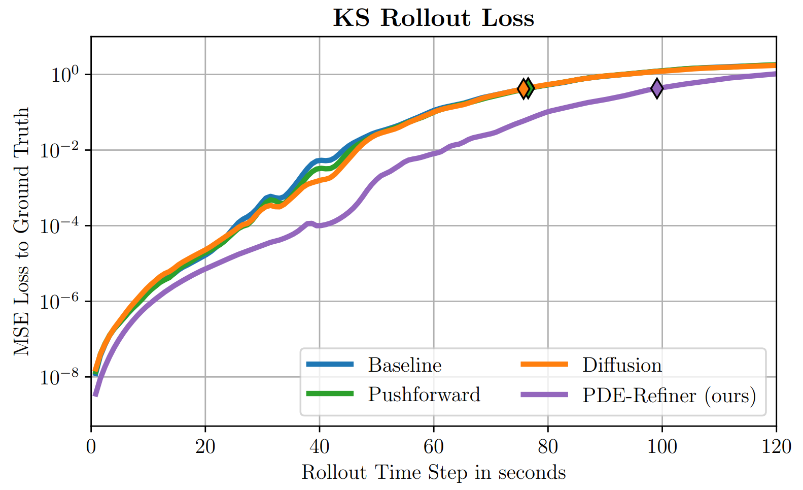
We compare PDE-Refiner to several neural operators and training methods on the 1D Kuramoto-Sivashinsky equation, with the results above using U-Nets and results for FNO can be found in the paper. The standard operator training maintains accurate predictions up to 75 seconds, whereby even increasing the parameters by 4 times only improves performance by 5 seconds. Alternative losses and training methods, like the pushforward trick, similarly do not improve the performance. In contrast, PDE-Refiner obtains accurate predictions up to almost 100 seconds, which is a 30% improvement over the standard neural operator. Even with a single refinement steps, we gain 15 seconds, showing the importance of modeling all frequencies well. The number of steps therefore gives us a way to trade-off between accuracy and speed, depending on what is most important in the application.

Results of evaluating several neural operators and training methods on the KS equation. Light and dark colors show the rollout time at which the correlation between the prediction and ground truth drops below 0.8 and 0.9 respectively.

Furthermore, when analysing the frequency spectrum of the predictions, we can see that PDE-Refiner indeed models a much larger band of frequencies accurately. This is also reflected in the loss over rollout, where PDE-Refiner has initially a similar loss as the standard operator, but then maintains a much lower loss for longer. Finally, we can see that PDE-Refiner is able to accurately estimate its own uncertainty by repeating the refinement process with different sampled noise, which is important for many applications. Click through the carousel below to see more results!

PDE-Refiner's frequency spectrum is accurate for a much larger range compared to the standard neural operator training, while achieving similar accuracy for the dominating frequency. Note that not only high frequencies, but even the lowest few frequencies improve due to their lower amplitude than the dominating one.

The refinement steps of PDE-Refiner focus on different amplitude ranges. While the first step has a similar frequency spectrum as the standard neural operator, it improves significantly for the high frequencies over the next steps. Meanwhile, the dominating one does not improve much beyond refinement step 2.

Recording the loss over time in the rollouts reveals that PDE-Refiner is very similar to the standard neural operator in the first 20 seconds. Afterwards, it starts to significantly diverge from the ground truth solution, while PDE-Refiner maintains a lower loss for much longer due to it modeling the high frequencies.

Uncertainty estimation is performed by sampling multiple trajectories from PDE-Refiner, and comparing their cross-correlation to the correlation to the actual ground truth solution. The estimates closely match the ground truth correlation, even per sample, allowing us to estimate when to fall back to numerical solvers again.

Experiments - 2D Kolmogorov Flow

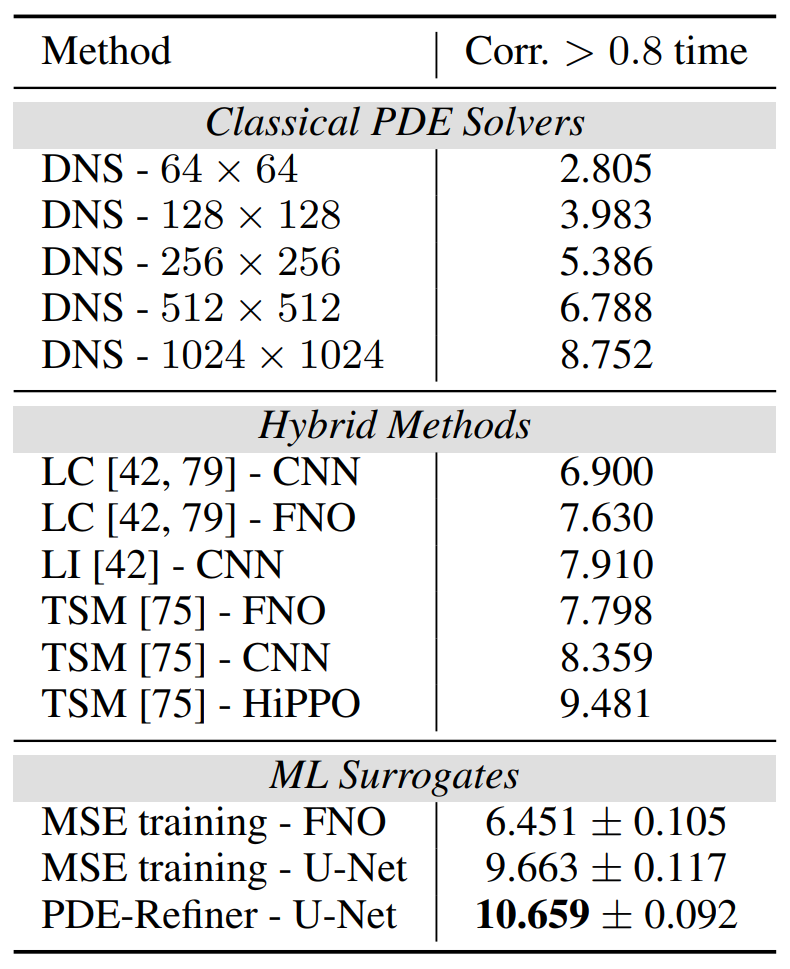
Besides the Kuramoto-Sivashinsky equation, we also evaluate PDE-Refiner on the 2D Kolmogorov flow, which is a variant of the incompressible Navier-Stokes equation. This equation is known for its chaotic behavior for high Reynolds numbers, which makes it a challenging benchmark for neural PDE solvers. Due to that, the numerical solvers we use for generating the ground truth data operate on a resolution of 2048x2048 pixels, while we train our neural operators on a resolution of 64x64 pixels. We compare PDE-Refiner not only to other neural operators, but also classical numerical and state-of-the-art hybrid solvers.

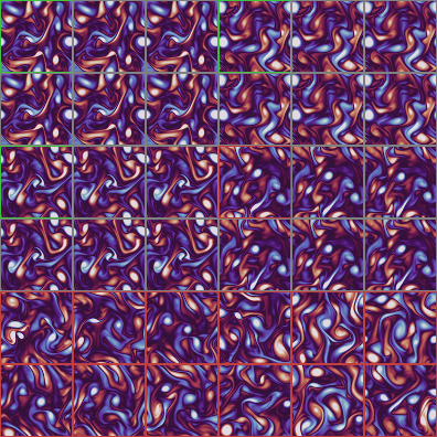
The results on the right show that PDE-Refiner obtains accurate predictions up to 10.6 seconds, outperforming other neural operators as well as the hybrid solver. Furthermore, despite its refinement process, PDE-Refiner is still faster than the best hybrid solver, giving more accurate and faster predictions. Meanwhile, the numerical solver at 2048x2048 pixels is more than 100x slower than PDE-Refiner, showing the benefit of neural operators. Finally, PDE-Refiner is again able to estimate its uncertainty well, despite being slighlty overconfident due to the small dataset. The GIF below shows the ground truth on the top left, along with 5 predictions of PDE-Refiner. The border turning red on the ground truth indicates the times when the correlation to the ground truth drops below 0.8, with the border of the predictions showing the cross-correlation. Check out the paper for more details!

Trajectories of PDE-Refiner on the 2D Kolmogorov Flow. PDE-Refiner remains accurate for over 10 seconds, while estimating its uncertainty by the cross-correlation between samples.

Want to learn more about PDE-Refiner?

Check out our paper!

Paper Code Datasets Poster Video

BibTeX


@inproceedings{lippe2023pderefiner,
  title        = {{PDE-Refiner: Achieving Accurate Long Rollouts with Temporal Neural PDE Solvers}},
  author       = {Phillip Lippe and Bastiaan S. Veeling and Paris Perdikaris and Richard E Turner and Johannes Brandstetter},
  year         = 2023,
  booktitle    = {Thirty-seventh Conference on Neural Information Processing Systems},
  url          = {https://openreview.net/forum?id=Qv6468llWS}
}

PDE-Refiner: Achieving Accurate Long Rollouts with Neural PDE Solvers

PDE-Refiner modeling the 1D Kuramoto-Sivashinsky Equation

Each line represents a predicted trajectory sampled from PDE-Refiner, with the average correlation to the ground truth and across samples shown on the right. PDE-Refiner obtains long accurate rollouts while providing accurate uncertainty estimates.